SELECT * FROM knowledge: An Intro to SQL

If you are stepping into the world of data, you have probably heard of SQL (Structured Query Language). It is the standard language for communicating with databases.

I recently completed my SQL training within the Data School and I want to share the core concepts I learned. Whether you are a total beginner or just need a refresher, here is a breakdown of how to query data, moving from simple commands to advanced analysis.

1. The Basics: Retrieving Your Data

The most fundamental command in SQL is SELECT. You use this to tell the database which columns you want, and FROM to tell it which table to look in.

The Basic Select

To see everything in a table, we use the wildcard *.

SQL

-- Select all columns from customers table.
SELECT 
*
FROM customers;

Pro Tip: In the real world, tables can have millions of rows. It is good practice to peek at the data without loading everything by using LIMIT.

SQL

-- Limit to 50 rows
SELECT 
*
FROM customers
LIMIT 50;

Renaming Columns

Sometimes column names in a database are messy (e.g. cust_id). You can use AS to rename them in your results to make them readable.

SQL

-- Renaming columns for better readability
SELECT
    order_id AS "Order ID"
    ,order_date AS "Order Date"
FROM orders;

2. Filtering: Finding What You Need

Rarely do we need all the data. Usually, we are looking for something specific. This is where the WHERE clause comes in.

Exact Matches and Ranges

We can filter by numbers, ranges, or specific text.

SQL

-- Sales between 50 and 100 AND ship mode is Second Class
SELECT
    SALES
    ,SHIP_MODE
FROM orders
WHERE sales BETWEEN 50 AND 100
  AND SHIP_MODE = 'Second Class';

Pattern Matching

What if you don't know the exact spelling, or you want everyone from a specific region?

LIKE: Uses wildcards. %town finds "Georgetown", "Jamestown", etc.
IN: A cleaner way to say "OR this OR that".

SQL

-- Customers where city ends in 'town'
SELECT
    city
    ,customer_name
FROM customers
WHERE city LIKE '%town';

-- Customers from specific states
SELECT
    state
    ,customer_name
FROM CUSTOMERS
WHERE state IN ('Texas', 'Oregon', 'New York');

3. Joining Tables: The Heart of SQL

Data is rarely stored in one big spreadsheet. It is usually split into tables (like Orders, Customers, Products) to save space. To analyse them together, we need Joins.

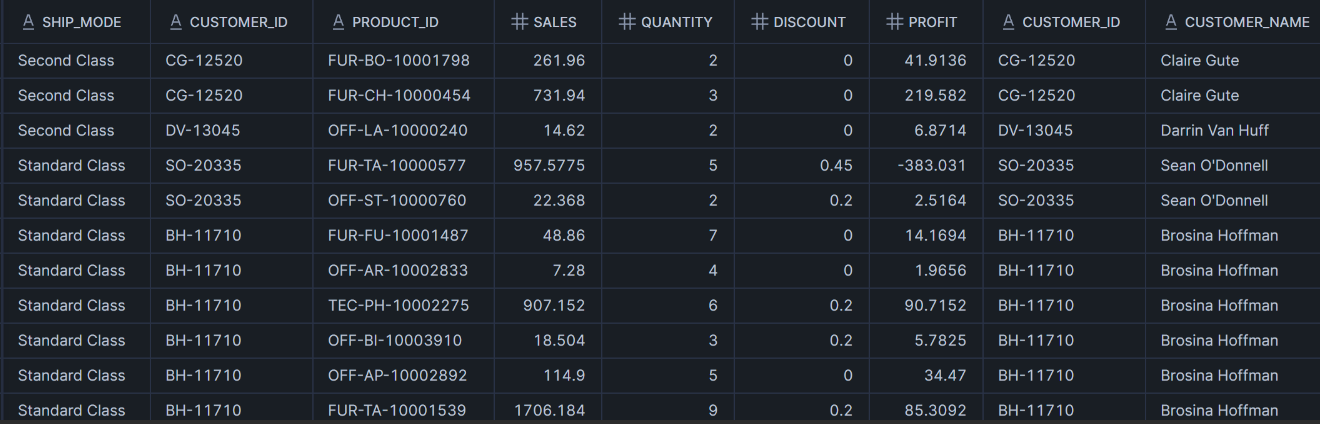
Left Join

This is the most common join. It keeps everything from the left table (Orders) and brings in matching details from the right table (Customers).

SQL

-- Join Orders and Customers
SELECT
    *
FROM orders o
LEFT JOIN customers c
    ON o.customer_id = c.customer_id;

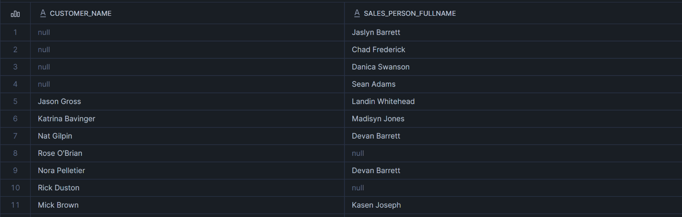
Full Join (The "Catch-All")

A full join returns combines all records from both tables, returning all matching rows and also including unmatched rows from either table, filling the missing data with NULL values. This is great for finding missing links.

Exercise: We wanted to find sales reps with no customers, or customers with no sales reps.

SQL

SELECT
    customer_name
    ,sales_person_fullname
FROM customers c
FULL JOIN customer_sales_rep csr
    ON c.customer_id = csr.customer_id;

4. Aggregation: Summarising the Numbers

Data analysis isn't just about listing rows; it's about summarising them.

Basic Math

We can sum, count, or find averages easily.

SQL

-- Total sales across the company
SELECT
    SUM(sales) AS total_sales
FROM orders;

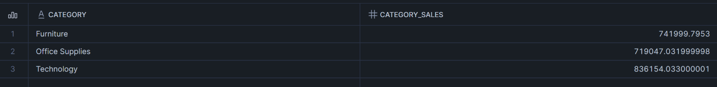
Grouping Data

To see sales per category or per state, we use GROUP BY.

SQL

-- Sales by Product Category
SELECT
    category
    ,SUM(sales) AS category_sales
FROM orders o
LEFT JOIN products p
    ON o.product_id = p.product_id
GROUP BY category;

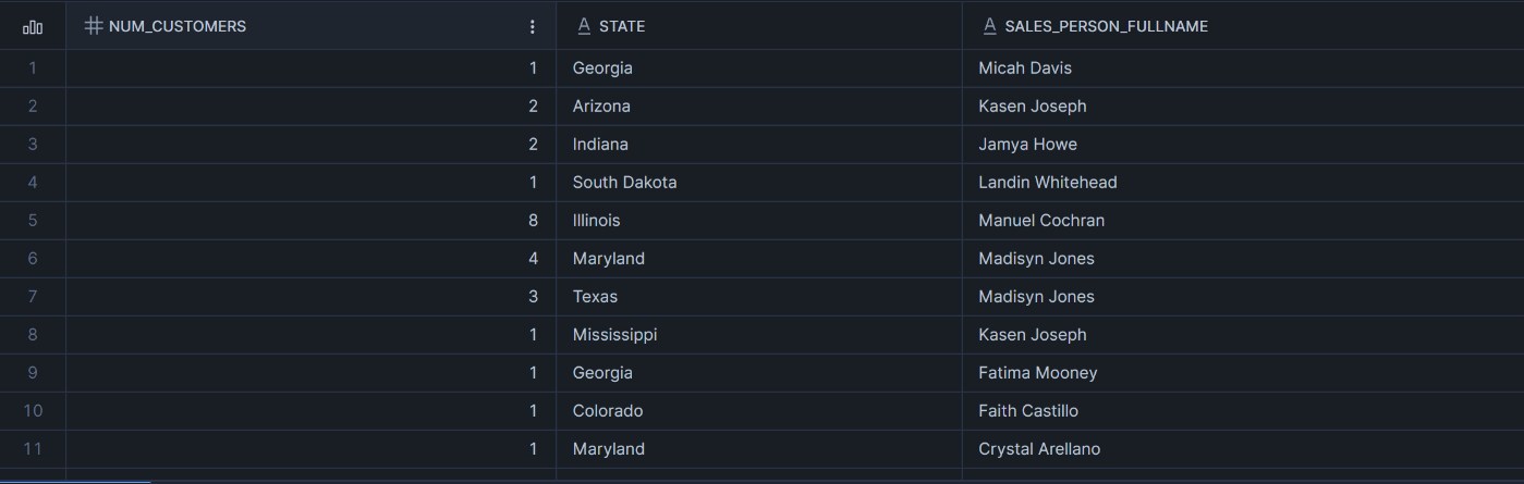
The "Distinct" Count

Sometimes a customer places 10 orders. If we want to know how many unique customers we have, we use DISTINCT.

SQL

-- Distinct count of customers per state and sales person
SELECT
    COUNT(DISTINCT c.customer_id) AS num_customers
    ,state
    ,sales_person_fullname
FROM customers c
JOIN customer_sales_rep crp
    ON c.customer_id = crp.customer_id
GROUP BY state, sales_person_fullname;

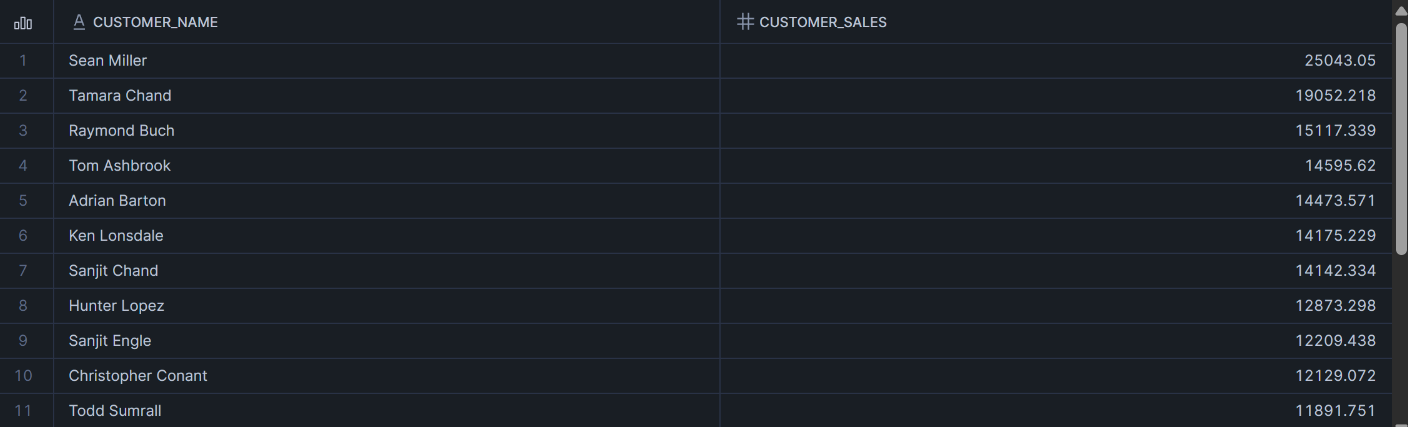
Filtering Aggregations (`HAVING`)

Important distinction: Use WHERE to filter raw rows. Use HAVING to filter after you have grouped and calculated data.

SQL

-- Customers with TOTAL sales > 10,000
SELECT
    customer_name
    ,SUM(sales) AS customer_Sales
FROM orders o
LEFT JOIN customers c
    ON o.customer_id = c.customer_id
GROUP BY customer_name
HAVING SUM(sales) > 10000
ORDER BY customer_Sales DESC;

5. Advanced SQL: Subqueries vs. CTEs

Finally, I tackled how to answer complex questions, like: "What percentage of total sales does each category represent?"

To do this, you need two numbers at once:

The sales for the category.
The sales for the whole company.

Option 1: The Subquery

A subquery is a query nested inside another query.

SQL

-- Sub-Query
SELECT
    category
,sum(sales) as category_sales
,category_sales/
(
select
    sum(sales) as total_sales
from orders
) as pct_total_sales
from orders o
inner join products p
on o.product_id = p.product_id
group by category;

Option 2: Common Table Expressions (CTE)

CTEs are often preferred because they are more readable. You define the "helper" data first, then run your main query.

SQL

-- Calculate total sales first
WITH total_sales_cte AS (
    SELECT
        SUM(sales) AS total_sales
    FROM orders
)

-- Then use it in the main query
SELECT
    category
    ,SUM(sales) AS category_sales
    ,SUM(sales) / MAX(total_sales) AS pct_total
FROM orders o
INNER JOIN products p
    ON o.product_id = p.product_id
CROSS JOIN total_sales_cte
GROUP BY category;

Conclusion

SQL is incredibly powerful. Starting from a simple SELECT *, I learned how to slice, dice, and summarise complex datasets. While the syntax can look intimidating at first, it follows a logical structure that becomes second nature with practice.

Author:

Robin Jones

View Profile