


A few weeks into training at The Data School, our cohort was given an assignment. Each of us was assigned a folder from Tableau’s calculated field function library and tasked with becoming an expert on it. My folder was Aggregate. The goal was simple: learn it well enough to explain it to someone else. While this initially was only a class assignment, I began to realize it could be something useful to share with others!
I wanted to polish my work and put this together because honestly, I wish something like this had existed when I first opened Tableau. To clarify, the documentation existed but it was not always written in a way that clicked for me right away. If you are in the middle of your first project or just starting to explore calculated fields, think of this as a plain English starting point from someone who just went through the learning curve themselves.
Before we get into it, two quick terms worth knowing:
A calculated field is a new field you create inside Tableau using a formula. Think of it like writing a formula in Excel, except it lives inside your visualization.
An aggregate function is a type of formula that summarizes across multiple rows and returns a single value, like a total, an average, or a count, rather than looking at one row at a time.
There are 21 aggregate functions in Tableau. I grouped them into categories to make them easier to digest.
General Functions
ATTR - Use this to check whether all rows in a group share the same value for a field. Returns that value if they do, an asterisk if they don’t.
Formula: ATTR([Field])
CORR - Use this when you want to measure the mathematical relationship between two variables, somewhat similar to the R-squared value you see when adding a trend line to a scatter plot.
Formula: CORR([Field 1], [Field 2])
COUNT - Use this to count how many rows exist in a group. Nulls are ignored.
Formula: COUNT([Field])
COUNTD - Use this when you want to know how many unique values exist in a group rather than just how many rows. Nulls are ignored.
Formula: COUNTD([Field])
MAX - Use this to find the largest value in a column, or to compare two fields row by row and return whichever is higher.
Formula: MAX([Field]) or MAX([Field 1], [Field 2])
MIN - Use this to find the smallest value in a column, or to compare two fields row by row and return whichever is lower.
Formula: MIN([Field]) or MIN([Field 1], [Field 2])
PERCENTILE - Use this to see where a value ranks relative to the rest of the dataset. For example, PERCENTILE([Sales], 0.60) returns the value below which 60% of your sales figures fall. The decimal must be between 0 and 1.
Formula: PERCENTILE([Numeric Field], [Decimal Number])
Level of Detail (LOD) Expressions
One of the most important concepts I picked up at The Data School is granularity: understanding what each row in your dataset actually represents and how that changes depending on how you look at it. LOD expressions are where that concept becomes a tool. They let you control the granularity of a calculation independently of what is on your sheet, which means you can ask questions at a different level of detail than what Tableau is currently displaying. I have not used these extensively yet but I expect they will become some of the most reached for functions as my work gets more complex.
EXCLUDE - Removes a specific dimension from the calculation, effectively changing the level of detail.
Formula: { EXCLUDE [Dimension] : SUM([Measure]) }
FIXED - Locks the calculation to a specific dimension regardless of what else is on the sheet.
Formula: { FIXED [Dimension] : SUM([Measure]) }
INCLUDE - Adds a dimension into the calculation even if it is not currently visible on the sheet.
Formula: { INCLUDE [Dimension] : SUM([Measure]) }
Numeric Fields Only
AVG - Use this to return the average of all values in a field. Nulls are ignored.
Formula: AVG([Numeric Field])
MEDIAN - Use this instead of AVG when your data has extreme highs or lows that could skew the average. Nulls are ignored.
Formula: MEDIAN([Numeric Field])
SUM - Use this to add up all values in a field. Nulls are ignored.
Formula: SUM([Numeric Field])
Spatial Fields Only
COLLECT - Use this to group all spatial data points into a single collection while keeping their individual borders intact.
Formula: COLLECT([Spatial Field])
UNION - Use this to dissolve the borders between neighboring map shapes and fuse them into one. Different from COLLECT which groups but preserves borders.
Formula: UNION([Spatial Field])
Sample vs. Population Functions
This is where things get a little statistical. Each of these functions comes in two versions: one for samples and one for populations. You would use the sample version when your data represents a sample of a larger population, and the population version when your dataset contains the entire population you want to analyze.
COVAR - Use this to measure whether two variables tend to move in the same direction or opposite directions.
Formula: COVAR([Field 1], [Field 2])
COVARP - Does the same as COVAR but treats the data as the full population.
Formula: COVARP([Field 1], [Field 2])
STDEV - Use this to measure how spread out your values are around the average. Imagine a train that averages a 10 minute wait. An STDEV of 1 means it is reliably on time. An STDEV of 8 means you have no idea when it is showing up.
Formula: STDEV([Numeric Field])
STDEVP - Does the same as STDEV but treats the data as the full population.
Formula: STDEVP([Numeric Field])
VAR - Use this to measure how far values stretch from their average, similar to STDEV but without the final square root step. Low variance means consistent, high variance means unpredictable.
Formula: VAR([Numeric Field])
VARP - Does the same as VAR but treats the data as the full population.
Formula: VARP([Numeric Field])
What You Can Actually Build With These
The reason I found this assignment so valuable is that these functions are not abstract. They show up the moment you try to do anything beyond a basic chart.
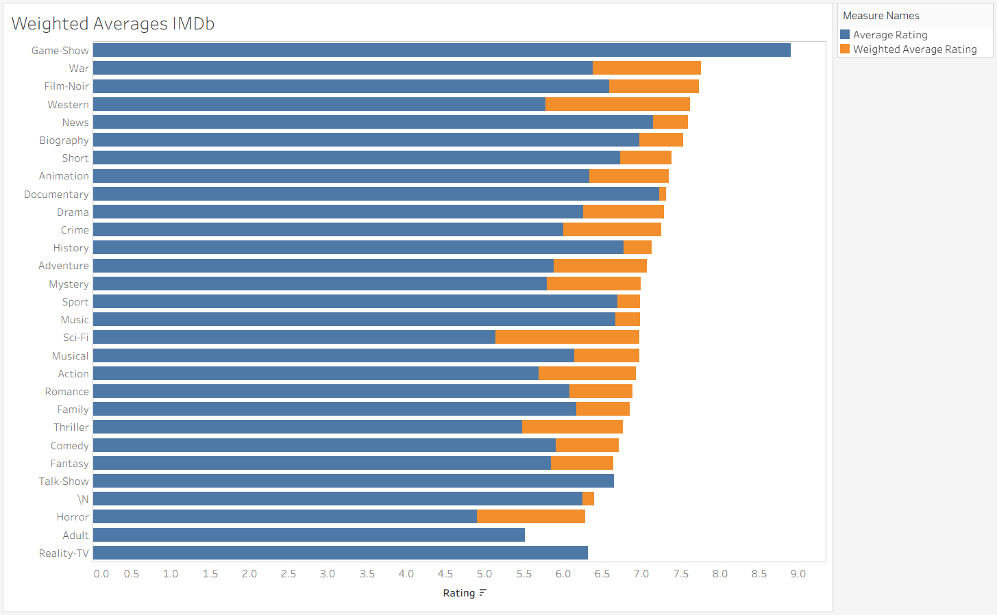
Take weighted averages. A simple AVG treats every row equally regardless of how many votes or responses it represents. A weighted average accounts for that. Here is the formula I used on an IMDb dataset we worked on the same day:
SUM([Average Rating] * [Num Votes]) / SUM([Num Votes])
The chart below shows the difference between a straight average rating and a weighted average rating across film genres. Notice how much the picture changes once you account for volume.
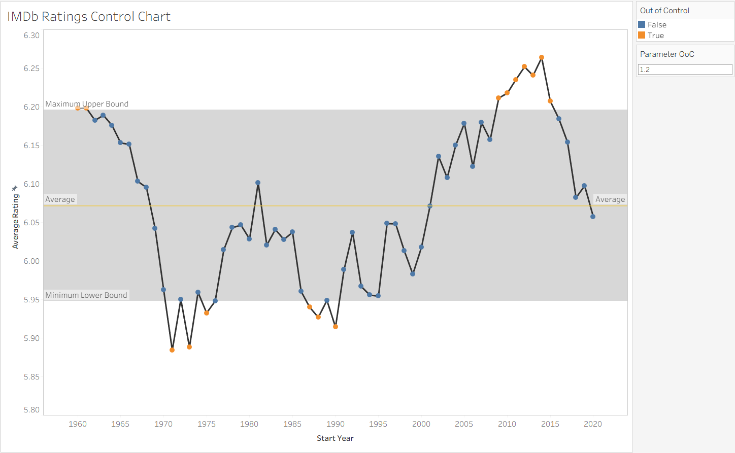
Then there is the control chart, which uses STDEV to flag data points that fall outside a normal range. I built one tracking IMDb ratings over time. The orange points are out of control, meaning they deviate significantly from the historical average. The formula behind it:
AVG([Average Rating]) > ([Parameter OoC] * WINDOW_STDEV(AVG([Average Rating])) + WINDOW_AVG(AVG([Average Rating])))
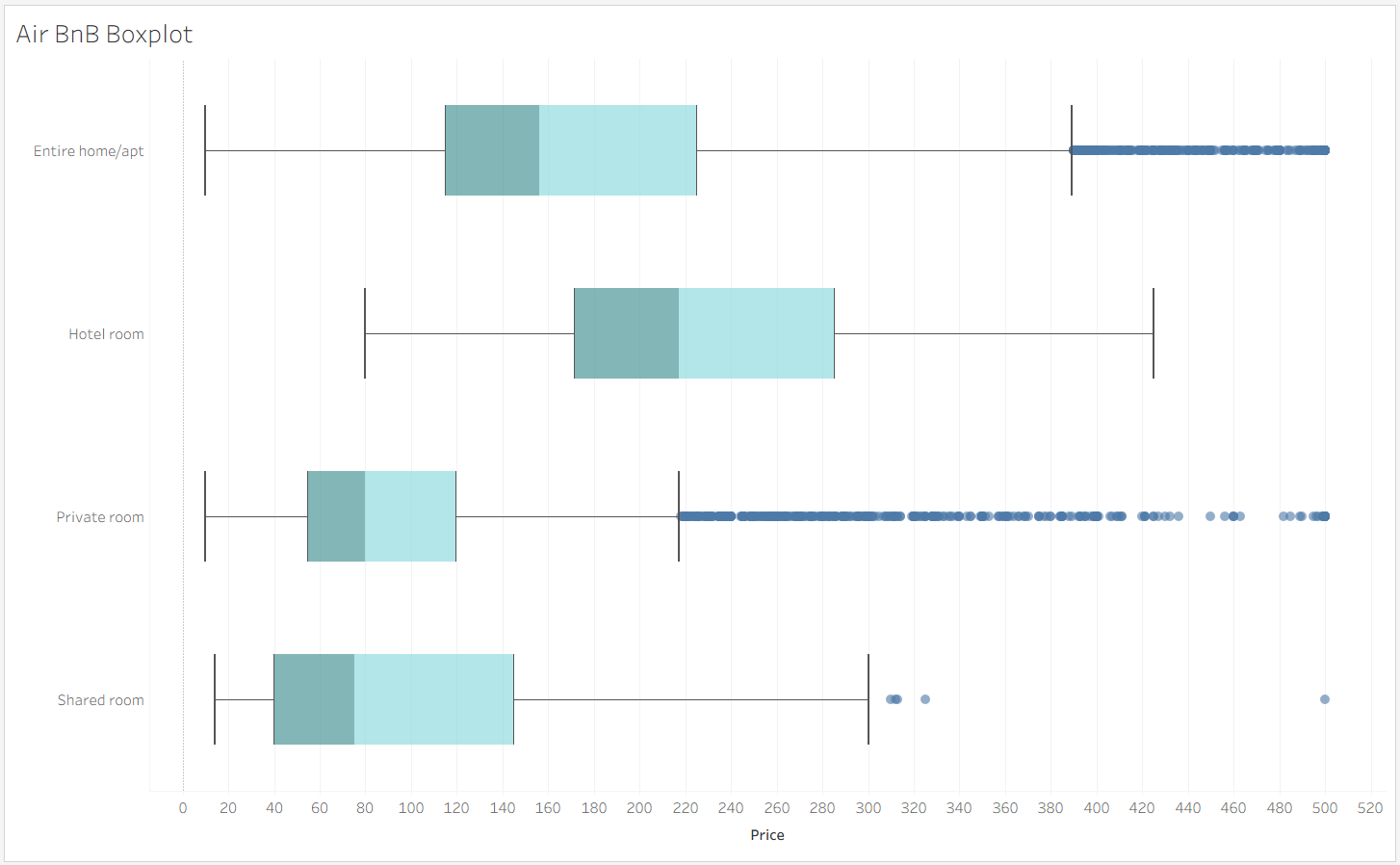
And finally the box plot, which uses MEDIAN and percentile logic to show the full distribution of a dataset rather than just a single summary number. I applied it to Airbnb pricing data across room types. You can immediately see not just the average price but where the bulk of listings actually fall and how far the outliers stretch.
What the Assignment Taught Me
This assignment reminded me of something that goes beyond Tableau. Being handed a topic and told to become the expert on it fast is exactly what consulting asks of you. You will not always have weeks to prepare. Sometimes you have an afternoon. In those situations we cannot panic, we have to put the effort in and get the work done. Use the resources available, whether that is a search engine, the Tableau documentation, or simply the person sitting next to you.
That last one is something I have come to appreciate more than I expected. Being part of The Information Lab means having a community of people who have been in your exact position and are genuinely willing to help you work through it. The blogs, the coaches, the consultants, even my own cohort, all of it has made the learning curve feel a lot less steep. If you are applying to The Data School or just starting out with Tableau, lean into that. The tools are learnable. The community is what makes it stick.